13.5 Factor rotation and interpretation of EFA
To perform EFA we will use the function fa() from the package psych. This function allows us to select the factoring method for the extraction of factors (e.g., minimum residual, maximum likelihood, weight least squares). We will use ml because the maximum likelihood algorithm finds the communality values that minimize the chi-square goodness of fit, assuming normality in continuous indicators. We must specify the number of factors to extract (in our example, two factors). We can enter this argument (nfactors = 2) because we have computed a parallel analysis in the previous section. The last important argument to set is the factor rotation (rotate).
Why do we rotate factors?
The main reason to rotate factors is to favor its interpretation by producing the simplest structure of the factor loadings. There are two types of factor rotations: orthogonal and oblique rotations (Figure 13.8).
The orthogonal rotation assumes that factors are independent (i.e., uncorrelated). Consequently, the axes remain perpendicular as they rotate. In psychology, it is very uncommon to deal with independent factors. However, there is considerable amount of evidence supporting the orthogonal and bidimensional structure of affect (i.e., core affect) (Russell, 1980, 2003). For orthogonal rotations, varimax and quartimax are the most common methods.
On the other hand, oblique rotations allow factors to correlate. Consequently, the axes are not perpendicular when rotated. We prefer using the oblique rotation oblimin instead of other popular methods such as promax and quartimin.
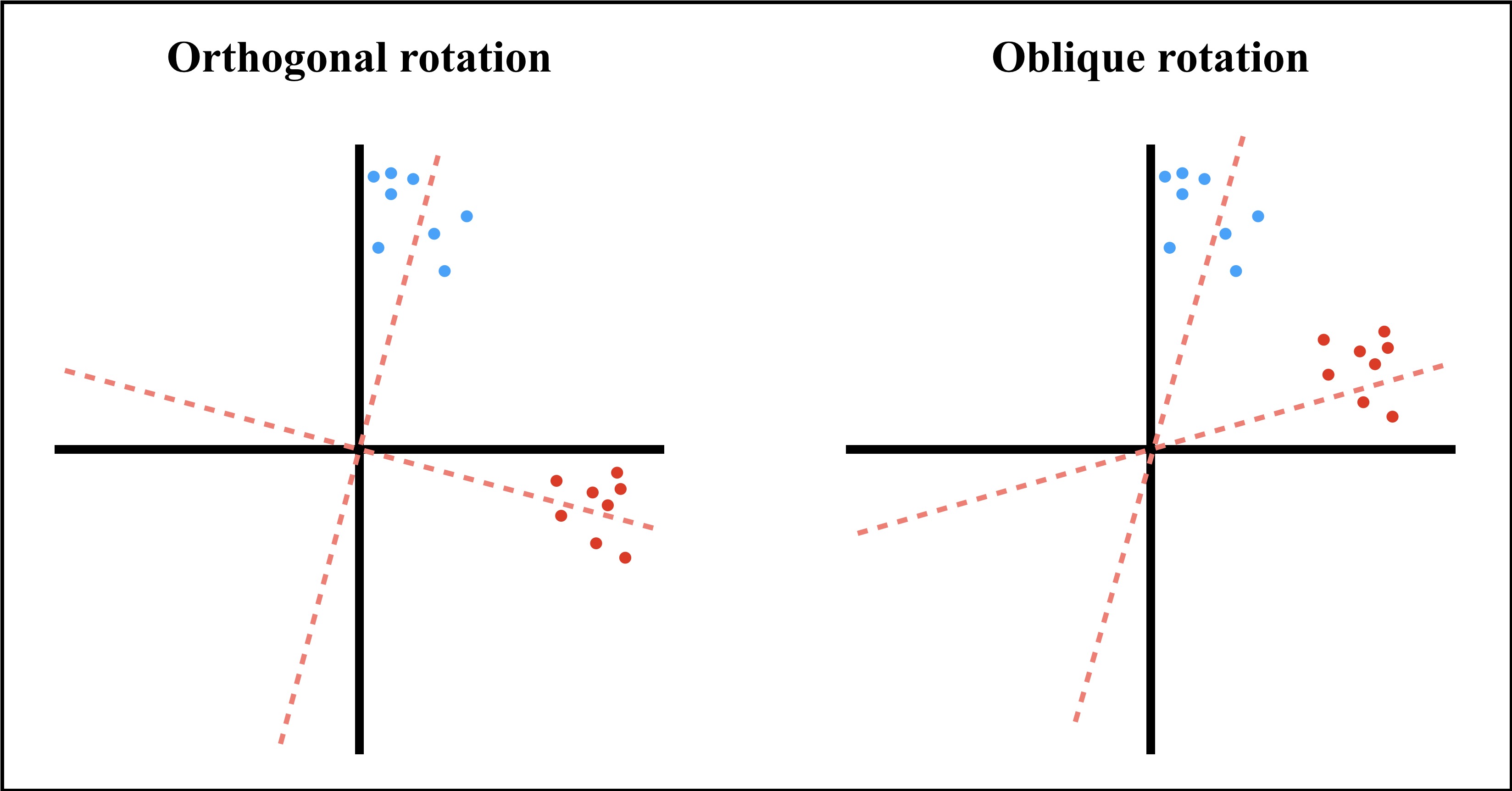
Figure 13.8: Orthogonal and oblique rotations.
burnout.fa <- fa(corre, nfactors = 2, rotate = 'oblimin', scores = 'regression',
                 fm = 'ml')
summary(burnout.fa)
##
## Factor analysis with Call: fa(r = corre, nfactors = 2, rotate = "oblimin", scores = "regression",
##     fm = "ml")
##
## Test of the hypothesis that 2 factors are sufficient.
## The degrees of freedom for the model is 43  and the objective function was  0.34
##
## The root mean square of the residuals (RMSA) is  0.05
## The df corrected root mean square of the residuals is  0.06
##
##  With factor correlations of
##      ML2  ML1
## ML2 1.00 0.37
## ML1 0.37 1.00

print(burnout.fa, sort = TRUE)
## Factor Analysis using method =  ml
## Call: fa(r = corre, nfactors = 2, rotate = "oblimin", scores = "regression",
##     fm = "ml")
## Standardized loadings (pattern matrix) based upon correlation matrix
##     item   ML2   ML1   h2   u2 com
## i1     1  0.76 -0.04 0.56 0.44 1.0
## i8     8  0.68 -0.18 0.40 0.60 1.1
## i6     6  0.65  0.10 0.48 0.52 1.0
## i10   10  0.64  0.06 0.44 0.56 1.0
## i2     2  0.56  0.12 0.38 0.62 1.1
## i3     3  0.37  0.25 0.27 0.73 1.7
## i12   12  0.32  0.03 0.11 0.89 1.0
## i9     9  0.04  0.83 0.71 0.29 1.0
## i7     7 -0.01  0.80 0.64 0.36 1.0
## i11   11 -0.16  0.56 0.28 0.72 1.2
## i5     5  0.30  0.40 0.35 0.65 1.9
## i4     4  0.33  0.38 0.34 0.66 2.0
##
##                        ML2  ML1
## SS loadings           2.76 2.19
## Proportion Var        0.23 0.18
## Cumulative Var        0.23 0.41
## Proportion Explained  0.56 0.44
## Cumulative Proportion 0.56 1.00
##
##  With factor correlations of
##      ML2  ML1
## ML2 1.00 0.37
## ML1 0.37 1.00
##
## Mean item complexity =  1.3
## Test of the hypothesis that 2 factors are sufficient.
##
## The degrees of freedom for the null model are  66  and the objective function was  3.74
## The degrees of freedom for the model are 43  and the objective function was  0.34
##
## The root mean square of the residuals (RMSR) is  0.05
## The df corrected root mean square of the residuals is  0.06
##
## Fit based upon off diagonal values = 0.98
## Measures of factor score adequacy
##                                                    ML2  ML1
## Correlation of (regression) scores with factors   0.91 0.92
## Multiple R square of scores with factors          0.83 0.84
## Minimum correlation of possible factor scores     0.66 0.69
The results from the standardized loadings matrix are telling. The proportion of communality of one item regarding the latent variables is shown in the column \(h^2\), whereas \(u^2\) represents the uniqueness (the error term). The column showing the complexity (com) is illustrative of items whose factor loadings do not contribute primarily to one factor. For example, items 4 and 5 (i.e., i4 and i5) yielded the highest complexity values, with large factor loadings in both factors.
We must inspect the factor loadings of each item. Factor loadings greater than .30 (\(\lambda^2 > .30\)) represent good loadings. However, as we have seen with the index of complexity, factor loadings greater than .30 in at least two factors indicate that the item is problematic (e.g., i4).
After inspecting the items with factor loadings greater than the established cut-off point (\(\lambda^2 > .30\)) on one factor only, we must provide a label for each latent variable. This process is done inductively, and it is guided by the theory. For example, the items with high factor loadings in factor 2 (ML2) could be appraised as Affective items (i.e., items that cover the subdomain of affective burnout). On the other hand, the items that are a good reflection of factor 1 (ML1) could be related to a Reward component of job burnout.
After labeling the factors, we will substitute (rename) the names of the columns of the list containing the factor loadings (ML2 and ML1) with the new names (Affective and Reward).
colnames(burnout.fa$loadings)
## [1] "ML2" "ML1"
colnames(burnout.fa$loadings) <- c('Affective', 'Reward')
There is a better way to inspect our results if we use the function print(). We can specify the optional arguments cutoff (i.e., it only displays factor loadings greater than the cut-off point set at .30) and sort (e.g., if TRUE, all factor loadings are ordered).
print(loadings(burnout.fa), cutoff = .3, digits = 2, sort = TRUE)
##
## Loadings:
##     Affective Reward
## i1   0.76
## i2   0.56
## i6   0.65
## i8   0.68
## i10  0.64
## i7             0.80
## i9             0.83
## i11            0.56
## i3   0.37
## i4   0.33      0.38
## i5   0.30      0.40
## i12  0.32
##
##                Affective Reward
## SS loadings         2.65   2.07
## Proportion Var      0.22   0.17
## Cumulative Var      0.22   0.39
It seems that items 4 and 5 are problematic. These items should be dropped from the scale. Thus, we should re-run the EFA with the new subset of items (i.e., 10 items only). This process is iterative, and it will require a data-driven approach as it is an exploratory analysis.
To plot the results, we can generate a path diagram that will display the factorial structure of the Job Burnout Scale (Figure 13.9). The function fa.diagram() from the package psych can be customized to modify parameters such as the size of the ellipses surrounding the latent variables (e.size) or the squares of the observed variables (rsize). We can also set the cut-off point of the factor loadings to .30 or any other value to avoid displaying factor loadings smaller than the threshold set with the argument cut.
fa.diagram(burnout.fa,
           main = '\n Exploratory Factor Analysis (Job Burnout Scale)',
           labels = names(burnout), l.cex = 2, digits = 2,
           e.size = .05, rsize = 2.13, cut = .30, cex = 1.2, adj = 2)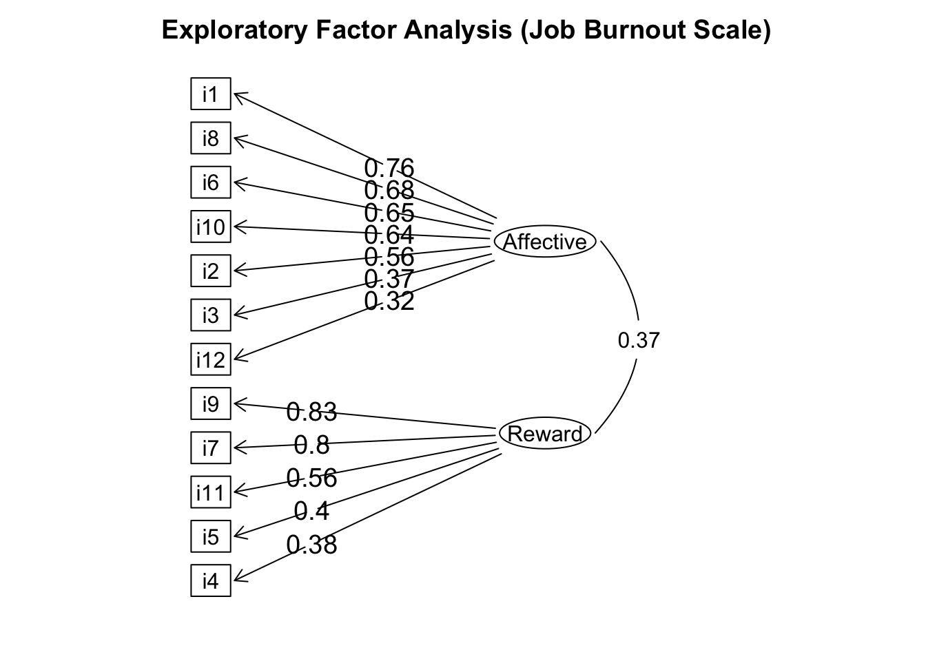
Figure 13.9: Path diagram (Job Burnout Scale).