13.3 Initial considerations
The scale's observed measures (i.e., the items) must be quantitative data. To estimate the correlations in the structure matrix (P), the scale needs to provide a sufficient amount of variability in the responses. As a rule of thumb, we will need at least 4-5 observed variables per factor and several hundred respondents to avoid underspecified models and a poor estimation of the internal structure of the scale (Fabrigar et al., 1999). Last, we will also require a significant number of high correlations (\(r > .30\)) among the items.
After collecting the data and selecting the observed variables (i.e., items) that we want to explore, we will organize and tidy the data set. For example, items negatively worded must be recoded. Likewise, we must check if there are missing cases (NaN) to drop them from the analyses.
Once the data set will be properly organized and formatted, we will generate the correlation matrix (P) and save it into an R object (e.g., the correlation matrix corre). Then, we will explore our data using some useful plots that will reveal the patterns of association, problematic issues regarding poor quality items, and an initial approximation to the latent variables of the scale.
13.3.1 Tidying the data set
In the current example, the Job Burnout Scale was used to measure 510 respondents' degree of agreement (5-point Likert scale: strongly disagree < disagree < neutral < agree < strongly agree) with the 12 statements covering the domain of the psychological construct job burnout. Two items were reversed worded (i3 and i8), requiring further recoding.
- Starting the session in R: Start every session in R by removing all objects from the global environment using the function
rm(). Likewise, set in advance the randomization seed for the current session using the functionset.seed(), and avoid using the scientific notation.
rm(list = ls())
set.seed(1234)
options(scipen=999)- Setting the working directory: Place the data set
burnout.savin the same folder where you will set the working directory. Then, set the working directory accordingly. For example, the instructor's working directory can be found in a folder named Chapter13 that is located inside of the folder LDSwR and the folder R; all of them placed in the home folder Users.
setwd('/Users/R/LDSwR/Chapter13')- Loading packages: Load the packages that will be required to execute the R code for this session.
library(rio)
library(dplyr)
library(psych)
library(corrplot)
library(skimr)- Reading the data set: To read the data from the SPSS file stored in the folder datasets inside of the working directory, use the function
import()from the package rio but do not forget to add the path with the additional folder (datasets) followed by the name of the data set with its corresponding file extension (e.g.,.sav,.csv,.dat). Given that there are 510 observations, it is not recommended to inspect all the rows of the data set. We could use the functionhead()to inspect the first six participants. We could also explore the dimensions of the data set (e.g., 510 rows and 23 columns) and the names of the variables using the functionsdim()andnames()respectively.
burnout.dat <- import('./datasets/burnout.sav')
head(burnout.dat)
##   id sex age i1 i2 i3 i4 i5 i6 i7 i8 i9 i10 i11 i12 burnoutTot stress job.satis
## 1  1   0  34  4  3  4  2  3  4  3  4  4   4   4   4         34     88        48
## 2  2   0  38  2  2  4  3  4  2  3  2  3   3   4   3         28     79        53
## 3  3   1  43  2  5  5  2  4  2  2  5  2   3   3   1         22     82        68
## 4  4   1  37  3  3  2  4  4  3  3  2  3   4   3   3         33     89        54
## 5  5   0  43  2  2  4  3  3  1  3  4  3   2   4   2         23     76        51
## 6  6   1  35  3  3  4  3  3  3  3  3  3   3   4   2         29     83        47
##   coping.skills contract
## 1            71        2
## 2            82        2
## 3            56        3
## 4            64        1
## 5            73        3
## 6            74        3
dim(burnout.dat)
## [1] 510  20
names(burnout.dat)
##  [1] "id"            "sex"           "age"           "i1"
##  [5] "i2"            "i3"            "i4"            "i5"
##  [9] "i6"            "i7"            "i8"            "i9"
## [13] "i10"           "i11"           "i12"           "burnoutTot"
## [17] "stress" "job.satis" "coping.skills" "contract"- Subsetting: To generate the correlation or structure matrix (P), we only need the 12 items of the Job Burnout Scale. For this reason, we are going to subset the data set to select the items 1 to 12 using the function
select()from the package dplyr. The resulting 12 covariates will be stored in a new R object namedburnout.
burnout <- burnout.dat %>%
  select(i1:i12)
headTail(burnout)
##      i1  i2  i3  i4  i5  i6  i7  i8  i9 i10 i11 i12
## 1     4   3   4   2   3   4   3   4   4   4   4   4
## 2     2   2   4   3   4   2   3   2   3   3   4   3
## 3     2   5   5   2   4   2   2   5   2   3   3   1
## 4     3   3   2   4   4   3   3   2   3   4   3   3
## ... ... ... ... ... ... ... ... ... ... ... ... ...
## 507   2   2   2   4   2   2   2   4   3   2   3   4
## 508   1   3   5   2   2   1   3   4   3   4   1   2
## 509   2   4   2   4   4   2   4   4   5   4   3   4
## 510   4   4   4   4   4   2   4   2   5   4   5   2
dim(burnout)
## [1] 510  12
names(burnout)
## [1] "i1" "i2" "i3" "i4" "i5" "i6" "i7" "i8" "i9" "i10" "i11" "i12"- Reverse scoring: We need to reverse the scoring of the two items that were negatively worded (
i3andi8). First, we will create a new vector (new) after selecting all the rows and only the columns of the items namedi3andi8. The vector namednewis the result of subtracting a value of6to the scores of two items that range from1to5. Consequently, a score of1will be transformed into a score of5(i.e.,6 - 1 = 5) and a score of5will be transformed into a score of1(i.e.,6 - 5 = 1). After reverse scoring the two items included in the vectornew, we will substitute the original itemsi3andi8included in our data set with the new ones stored in the R objectnew. As usual, you can inspect the result using the functionhead().
new <- 6 - burnout[ , c('i3', 'i8')]
burnout[ , c('i3', 'i8')] <- new
head(burnout)
##   i1 i2 i3 i4 i5 i6 i7 i8 i9 i10 i11 i12
## 1  4  3  2  2  3  4  3  2  4   4   4   4
## 2  2  2  2  3  4  2  3  4  3   3   4   3
## 3  2  5  1  2  4  2  2  1  2   3   3   1
## 4  3  3  4  4  4  3  3  4  3   4   3   3
## 5  2  2  2  3  3  1  3  2  3   2   4   2
## 6  3  3  2  3  3  3  3  3  3   3   4   2
13.3.2 Generating the correlation matrix
To conduct EFA, we can use the covariance or the correlation matrices. Here, we will use the correlation matrix (P; also called structure matrix). The function cor() generates the correlation matrix that we will store in the R object corre. In the first argument of the function cor(), we will input the data set that only includes the items. Although the second argument allows us to select among three different correlation methods (pearson, kendall, and spearman), the default option (pearson) is the one we need.
We will use the function na.omit() to avoid having missing observations. If these missing cases are not explicitly excluded from the analyses, we won't be able to generate the correlation matrix. To inspect the correlation matrix in the console simply recall the R object corre. The correlation matrix displayed below was produced with the package stargazer using the function stargazer() (Hlavac, 2018).
CAUTION!
We used the function stargazer() from the package stargazer within the Rmarkdown environment to produce a more appealing correlation matrix to the reader. It is important to set the argument results = 'asis' in the Rmarkdown code chunk to generate text as raw Markdown content.
corre <- cor(na.omit(burnout))
stargazer::stargazer(corre, type = 'html', rownames = T, summary = F,
                  digits = 2, header = F, font.size = 'Large',
                  column.sep.width = '7pt', align = T,
title = "Job Burnout Scale's Correlation Matrix.")| i1 | i2 | i3 | i4 | i5 | i6 | i7 | i8 | i9 | i10 | i11 | i12 | |
| i1 | 1 | 0.47 | 0.28 | 0.31 | 0.30 | 0.58 | 0.20 | 0.46 | 0.23 | 0.46 | 0.03 | 0.24 |
| i2 | 0.47 | 1 | 0.33 | 0.31 | 0.38 | 0.37 | 0.27 | 0.31 | 0.26 | 0.43 | 0.13 | 0.24 |
| i3 | 0.28 | 0.33 | 1 | 0.45 | 0.22 | 0.40 | 0.31 | 0.27 | 0.34 | 0.28 | 0.07 | 0.13 |
| i4 | 0.31 | 0.31 | 0.45 | 1 | 0.27 | 0.46 | 0.37 | 0.19 | 0.44 | 0.27 | 0.19 | 0.08 |
| i5 | 0.30 | 0.38 | 0.22 | 0.27 | 1 | 0.31 | 0.41 | 0.20 | 0.45 | 0.44 | 0.26 | 0.19 |
| i6 | 0.58 | 0.37 | 0.40 | 0.46 | 0.31 | 1 | 0.24 | 0.38 | 0.30 | 0.40 | 0.11 | 0.13 |
| i7 | 0.20 | 0.27 | 0.31 | 0.37 | 0.41 | 0.24 | 1 | 0.06 | 0.68 | 0.23 | 0.41 | 0.11 |
| i8 | 0.46 | 0.31 | 0.27 | 0.19 | 0.20 | 0.38 | 0.06 | 1 | 0.11 | 0.45 | -0.11 | 0.23 |
| i9 | 0.23 | 0.26 | 0.34 | 0.44 | 0.45 | 0.30 | 0.68 | 0.11 | 1 | 0.27 | 0.41 | 0.15 |
| i10 | 0.46 | 0.43 | 0.28 | 0.27 | 0.44 | 0.40 | 0.23 | 0.45 | 0.27 | 1 | 0.06 | 0.31 |
| i11 | 0.03 | 0.13 | 0.07 | 0.19 | 0.26 | 0.11 | 0.41 | -0.11 | 0.41 | 0.06 | 1 | 0.04 |
| i12 | 0.24 | 0.24 | 0.13 | 0.08 | 0.19 | 0.13 | 0.11 | 0.23 | 0.15 | 0.31 | 0.04 | 1 |
After generating the correlation matrix stored in corre, we will compute the Kaiser-Meyer-Olkin (KMO) test of factorial adequacy. To have a structure matrix appropriate for factor analysis, the overall KMO index should be greater than .80 and never below .70. The overall measure of sampling adequacy (MSA) was .85. Consequently, we can proceed with the factor analysis.
KMO(corre)
## Kaiser-Meyer-Olkin factor adequacy
## Call: KMO(r = corre)
## Overall MSA =  0.85
## MSA for each item =
##   i1   i2   i3   i4   i5   i6   i7   i8   i9  i10  i11  i12
## 0.84 0.90 0.87 0.87 0.89 0.85 0.80 0.85 0.80 0.88 0.82 0.87
13.3.3 Exploring the data using descriptive statistics and data visualizations
The function skim() from the package skimr provides a good summary of the items (i.e., the location, dispersion, and the form of the distribution).
skim(burnout)| Name | burnout |
| Number of rows | 510 |
| Number of columns | 12 |
| _______________________ | |
| Column type frequency: | |
| numeric | 12 |
| ________________________ | |
| Group variables | None |
Variable type: numeric
| skim_variable | n_missing | complete_rate | mean | sd | p0 | p25 | p50 | p75 | p100 | hist |
|---|---|---|---|---|---|---|---|---|---|---|
| i1 | 0 | 1 | 2.73 | 1.12 | 1 | 2 | 3 | 4 | 5 | ▃▇▅▅▁ |
| i2 | 0 | 1 | 3.36 | 1.08 | 1 | 2 | 4 | 4 | 5 | ▁▅▅▇▃ |
| i3 | 0 | 1 | 2.92 | 1.36 | 1 | 2 | 3 | 4 | 5 | ▅▇▃▇▅ |
| i4 | 0 | 1 | 3.10 | 1.25 | 1 | 2 | 3 | 4 | 5 | ▃▆▅▇▃ |
| i5 | 0 | 1 | 3.29 | 1.09 | 1 | 2 | 4 | 4 | 5 | ▁▃▃▇▂ |
| i6 | 0 | 1 | 2.46 | 1.15 | 1 | 2 | 2 | 3 | 5 | ▅▇▃▃▁ |
| i7 | 0 | 1 | 3.34 | 1.11 | 1 | 3 | 3 | 4 | 5 | ▁▅▆▇▃ |
| i8 | 0 | 1 | 2.78 | 1.19 | 1 | 2 | 2 | 4 | 5 | ▂▇▃▅▂ |
| i9 | 0 | 1 | 3.64 | 1.03 | 1 | 3 | 4 | 4 | 5 | ▁▂▅▇▃ |
| i10 | 0 | 1 | 3.57 | 0.99 | 1 | 3 | 4 | 4 | 5 | ▁▂▃▇▂ |
| i11 | 0 | 1 | 3.71 | 1.12 | 1 | 3 | 4 | 5 | 5 | ▁▂▃▇▅ |
| i12 | 0 | 1 | 3.63 | 1.04 | 1 | 3 | 4 | 4 | 5 | ▁▂▃▇▃ |
The function skim_with() from the package skimr enables us to specify our preferred list of descriptive statistics. We can also set the names of those statistics (e.g., we can display the APA abbreviation Mdn instead of median) or add other relevant descriptive statistics such as the Median Absolute Deviation (MAD).
my.summary <- skim_with(numeric = sfl(M = mean, SD = sd,
                                      Mdn = median, MAD = mad,
                                      Histogram = inline_hist), append = F)
my.summary(burnout)| Name | burnout |
| Number of rows | 510 |
| Number of columns | 12 |
| _______________________ | |
| Column type frequency: | |
| numeric | 12 |
| ________________________ | |
| Group variables | None |
Variable type: numeric
| skim_variable | n_missing | complete_rate | M | SD | Mdn | MAD | Histogram |
|---|---|---|---|---|---|---|---|
| i1 | 0 | 1 | 2.73 | 1.12 | 3 | 1.48 | ▃▇▁▅▁▅▁▁ |
| i2 | 0 | 1 | 3.36 | 1.08 | 4 | 1.48 | ▁▅▁▅▁▇▁▃ |
| i3 | 0 | 1 | 2.92 | 1.36 | 3 | 1.48 | ▅▇▁▃▁▇▁▅ |
| i4 | 0 | 1 | 3.10 | 1.25 | 3 | 1.48 | ▃▆▁▅▁▇▁▃ |
| i5 | 0 | 1 | 3.29 | 1.09 | 4 | 1.48 | ▁▃▁▃▁▇▁▂ |
| i6 | 0 | 1 | 2.46 | 1.15 | 2 | 1.48 | ▅▇▁▃▁▃▁▁ |
| i7 | 0 | 1 | 3.34 | 1.11 | 3 | 1.48 | ▁▅▁▆▁▇▁▃ |
| i8 | 0 | 1 | 2.78 | 1.19 | 2 | 1.48 | ▂▇▁▃▁▅▁▂ |
| i9 | 0 | 1 | 3.64 | 1.03 | 4 | 1.48 | ▁▂▁▅▁▇▁▃ |
| i10 | 0 | 1 | 3.57 | 0.99 | 4 | 1.48 | ▁▂▁▃▁▇▁▂ |
| i11 | 0 | 1 | 3.71 | 1.12 | 4 | 1.48 | ▁▂▁▃▁▇▁▅ |
| i12 | 0 | 1 | 3.63 | 1.04 | 4 | 1.48 | ▁▂▁▃▁▇▁▃ |
We use data visualization techniques to inspect relationships and patterns of association among items. For example, the function cor.plot() from the package psych (Revelle, 2018) shows a heatmap with red colors related to negative correlations and blue colors aimed at displaying the positive correlations. The functions corrplot.mixed() from the package corrplot or pairs.panels() from the package psych provide a lot of possibilities to visualize the correlation matrix stored in our R object named corre (see Figures 13.4, 13.5, and 13.6).
cor.plot(corre)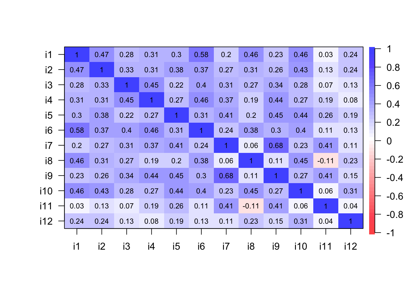
Figure 13.4: A correlation plot with heatmap.
You can add and modify as many arguments as you wish. For example, in the function corrplot.mixed(), number.cex reveals the character expansion value that enables the modification of the size of the numbers appearing in the plot, whereas tl.cex changes the size of the text labels (i.e., the names of the items that are displayed on the main diagonal of the correlation plot).
corrplot.mixed(corre, number.cex = 0.95, tl.col = 'orange4', tl.cex = 1.3,
               upper = 'square')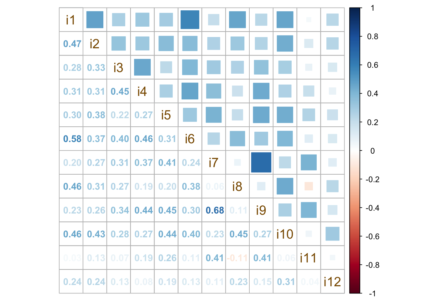
Figure 13.5: Mixed methods to visualize a correlation matrix.
The function pairs.panels() displays a scatter plot of matrices (SPLOM), with histograms on the main diagonal, and bivariate scatter plots and Pearson's correlations below and above the main diagonal. This plot works well with a small number of covariates.
pairs.panels(corre, hist.col = '#00AFBB', cex.cor = 1.10, cex.labels = 0.90,
               upper = 'square', lm = TRUE, show.points = TRUE, stars = TRUE,
               density = T, ci = TRUE)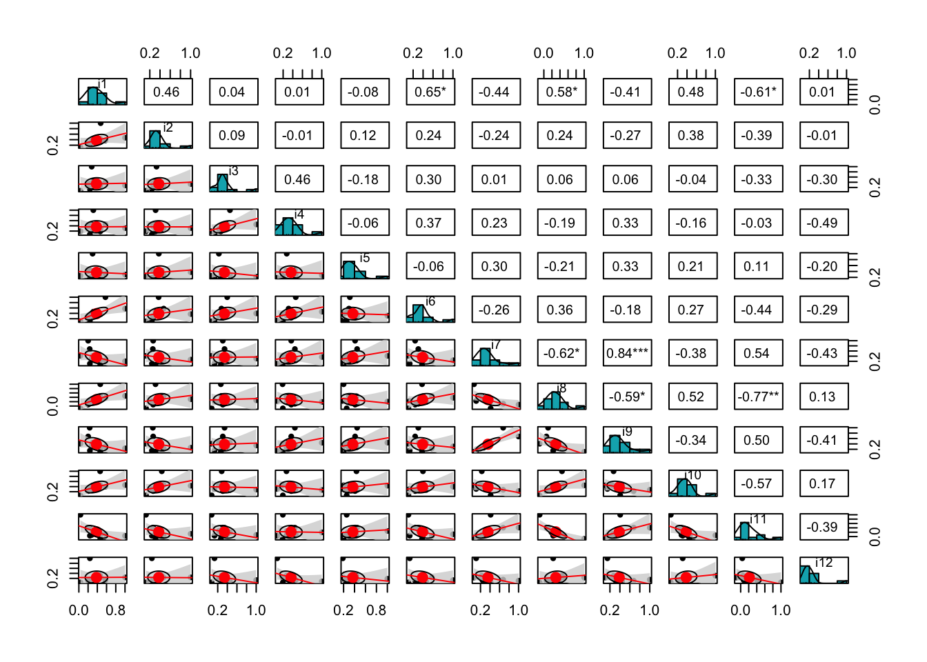
Figure 13.6: A scatter plot of matrices (SPLOM), with bivariate scatter plots, histograms, and Pearson's correlation.