14.3 Inter-rater reliability
Inter-rater reliability estimates the consistency among raters/judges (i.e., the agreement among raters). There are several methods to estimate inter-rater reliability. We can organize these methods as a function of the number of raters and the level of measurement. When we want to test the inter-rater reliability of two observers classifying objects or persons (i.e., nominal data), Cohen's Kappa (\(\kappa\)) would be the most appropriate method (Cohen, 1960). However, Fleiss's Kappa will be the preferred option for nominal data and more than two raters.
With ordinal data and two raters, estimating a Weight Kappa coefficient is recommended. On the other hand, Kendall's Tau-b test is the most appropriate test statistic to estimate the agreement of ordered objects or persons for multiple raters.
For quantitative data (e.g., interval data), the intraclass correlation (ICC) is the best method to measure the relative homogeneity of scores within a class (e.g., persons). The ICC estimates reliability using an Analysis of Variance (ANOVA) approach.
14.3.1 Cohen's Kappa
Cohen's Kappa (\(\kappa\)) estimates the degree of agreement between two raters/judges when assessing and classifying objects or persons (e.g., classification and diagnosis of mental disorders). This method is highly recommended because it considers the effect of random agreement. The agreement between two judges cannot be estimated by only counting the number of agreed cases (i.e., the main diagonal of a confusion matrix). We also need to subtract the estimation of the random agreement based on the marginal cross-products divided by the total number of squared observations.
To compute the observed agreement (\(p_{o}\)), we sum all the values from the main diagonal divided by the total number of observations.
\[\begin{aligned} \ p_{o} = \displaystyle\sum_{j=1}^{m} p_{jj} = \frac{N_{11}} {N} \ + \ \frac{N_{22}} {N} \ + \ \dots \ + \frac{N_{mm}} {N} \end{aligned}\]
To estimate the agreement due to randomness (\(p_{e}\)), we sum the marginal cross-products divided by the total number of squared observations.
\[\begin{aligned} \ p_{e} = \displaystyle\sum_{j=1}^{m} p_{jje} = \displaystyle\sum_{j=1}^{m} \frac{\ {N_{i}} \times {N_{j}}} {{N^{2}}} \end{aligned}\]
Cohen's Kappa (\(\kappa\)) is computed by subtracting the agreement due to randomness (\(p_{e}\)) to the observed agreement (\(p_{o}\)) divided by 1 minus the agreement due to randomness (\(p_{e}\)). The final inter-rater agreement coefficient will range from 0 to 1. Values in the .80 — 1 range are considered very good inter-rater reliability coefficients. Kappa's coefficients in the .60 — .79 range represent acceptable levels of agreement. However, agreement rates below .60 are usually considered unacceptable.
\[\begin{aligned} \ K = \frac{\ p_{o} \ - \ p_{e}} {1 \ - \ p_{e}} \end{aligned}\]
14.3.2 Cohen's Kappa in R
We will use the functions Kappa() and agreementplot() from the package vcd to compute Cohen's Kappa (\(\kappa\)) coefficients and to generate agreement plots for two different simulated data sets (Friendly, 2017).
library(vcd)The following simulated data sets will show the level of agreement between two clinical psychologists assessing and ascribing affective disorders to a group of 220 patients. Bi1 means Bipolar I disorder. Bi2 means Bipolar II disorder. PD means Persistent depressive. C means Cyclothymic. MD means Major depressive. We will generate two different matrices in which the observations (i.e., number of patients per cell) will be distributed along the main diagonal (i.e., agreement between raters) and off the main diagonal (i.e., disagreement between raters).
The first data set yields an inter-rater reliability of \(\kappa = .46, \ 95\% \ CI{[.38, \ .54]}\), that should be considered unacceptable. The function agreementplot() generates a representation of a k by k confusion matrix, where the observed and expected diagonal elements are represented by superposed black and white rectangles, respectively.
dat1 <- matrix(c(20, 27, 1, 3, 0,
                 23, 21, 0, 0, 0,
                 4, 2, 46, 1, 0,
                 2, 2, 0, 14, 17,
                 0, 0, 0, 13, 24), 5, 5, byrow = T,
                 dimnames= list(c('Bi1', 'Bi2', 'PD', 'C', 'MD'),
                                c('Bi1', 'Bi2', 'PD', 'C', 'MD')))
K1 <- Kappa(dat1)
print(K1, CI = TRUE)
##             value     ASE     z
## Unweighted 0.4574 0.04169 10.97
## Weighted   0.6774 0.02876 23.55
##                                                                                                                                   Pr(>|z|)
## Unweighted 0.00000000000000000000000000051798280819831024980496793930887936602748847277526847309482233086705226356508124929689529380993918
## Weighted   0.00000000000000000000000000000000000000000000000000000000000000000000000000000000000000000000000000000000000000000000000001148
##             lower  upper
## Unweighted 0.3757 0.5391
## Weighted   0.6210 0.7337

agreementplot(dat1, ylab = 'Rater 1', ylab_rot = 90, ylab_just = 'center',
              xlab = 'Rater 2', xlab_rot = 0, xlab_just = 'center',
              reverse_y = TRUE, weights = 1)
Figure 14.1: Agreement plot displaying low agreement between two clinical psychologists assessing individuals with affective disorders.
The second data set yields a very high inter-rater reliability, \(\kappa = .91, \ 95\% \ CI {[.87, \ .95]}\). The reason for such a high Kappa coefficient can be found in the small amount of disagreement between raters (i.e., there are very few cases in the off-diagonal cells).
dat2 <- matrix(c(79, 0, 0, 0, 0,
                 2, 31, 0, 0, 0,
                 1, 3, 46, 1, 0,
                 0, 2, 0, 6, 0,
                 0, 1, 0, 5, 43), 5, 5, byrow = T,
                 dimnames= list(c('Bi1', 'Bi2', 'PD', 'C', 'MD'),
                                c('Bi1', 'Bi2', 'PD', 'C', 'MD')))
K2 <- Kappa(dat2)
print(K2, CI = TRUE)
##             value     ASE     z Pr(>|z|)  lower  upper
## Unweighted 0.9087 0.02239 40.58        0 0.8648 0.9526
## Weighted   0.9457 0.01498 63.15        0 0.9163 0.9750

agreementplot(dat2, ylab = 'Rater 1', ylab_rot = 90, ylab_just = 'center',
              xlab = 'Rater 2', xlab_rot = 0, xlab_just = 'center',
              reverse_y = TRUE, weights = 1)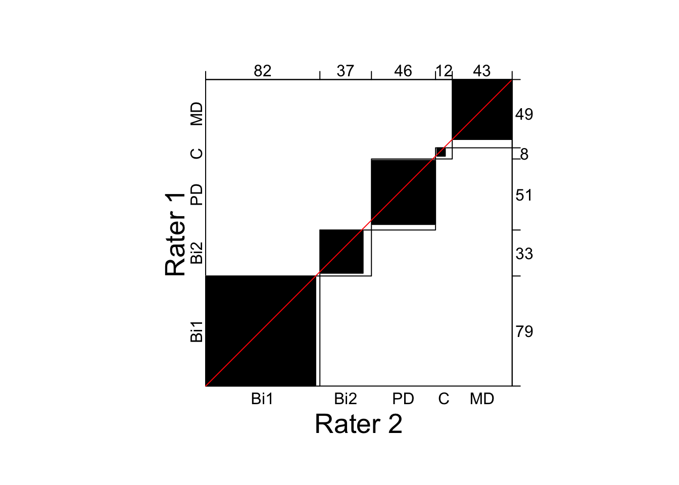
Figure 14.2: Agreement plot displaying high agreement between two clinical psychologists assessing individuals with affective disorders.