15.5 The Information Function
In psychometrics, the concept of information is related to the idea of precision with which a given ability/trait level (\(\theta\)) can be estimated. The amount of information (\(I\)) is inversely related to the size of the variability of the estimates around the value of a parameter (\(\sigma^{2}\)) (Baker & Kim, 2017).
\[\\I\ = \frac{1}{\sigma^{2}}\]
Thus, if the amount of information is small, the ability/trait cannot be estimated with precision (i.e., there will be a large variability of the estimates around the 'true' value of the parameter). In sum, the information function will show us how well each ability/trait level (\(\theta\)) is being estimated.
15.5.1 Item Information Function
Table 15.4 shows the parameter estimates computed on the 5-item test LSAT6 (Law School Admission Test, section 6) using a 2PL model (Chalmers, 2012; Thissen, 1982). Consequently, the additional parameters computed in 3PL (i.e., guessing) and 4PL (i.e., innatention) models were automatically constrained to 0 (i.e., no guessing) and 1 (i.e., no innatention) respectively.
Table 15.4 shows that item 3 is the most difficult item to answer (\(b_{j} = -0.28\)) and the one that discriminates the most (\(a_{j} = 0.89\)) between respondents with abilities above and below \(b_{j} = -0.28\). In contrast, item 5 is one of the easiest items of the test (\(b_{j} = -3.12\)) and it is also the least discriminant item (\(a_{j} = 0.66\)).
| Item | \(a_{j}\) | \(b_{j}\) | \(c_{j}\) | \(u_{j}\) |
|---|---|---|---|---|
| i1 | 0.83 | -3.36 | 0 | 1 |
| i2 | 0.72 | -1.37 | 0 | 1 |
| i3 | 0.89 | -0.28 | 0 | 1 |
| i4 | 0.69 | -1.87 | 0 | 1 |
| i5 | 0.66 | -3.12 | 0 | 1 |
| Note. \(a_{j}\) = Discrimination. \(b_{j}\) = Difficulty. \(c_{j}\) = Guessing. \(u_{j}\) = Inattention. |
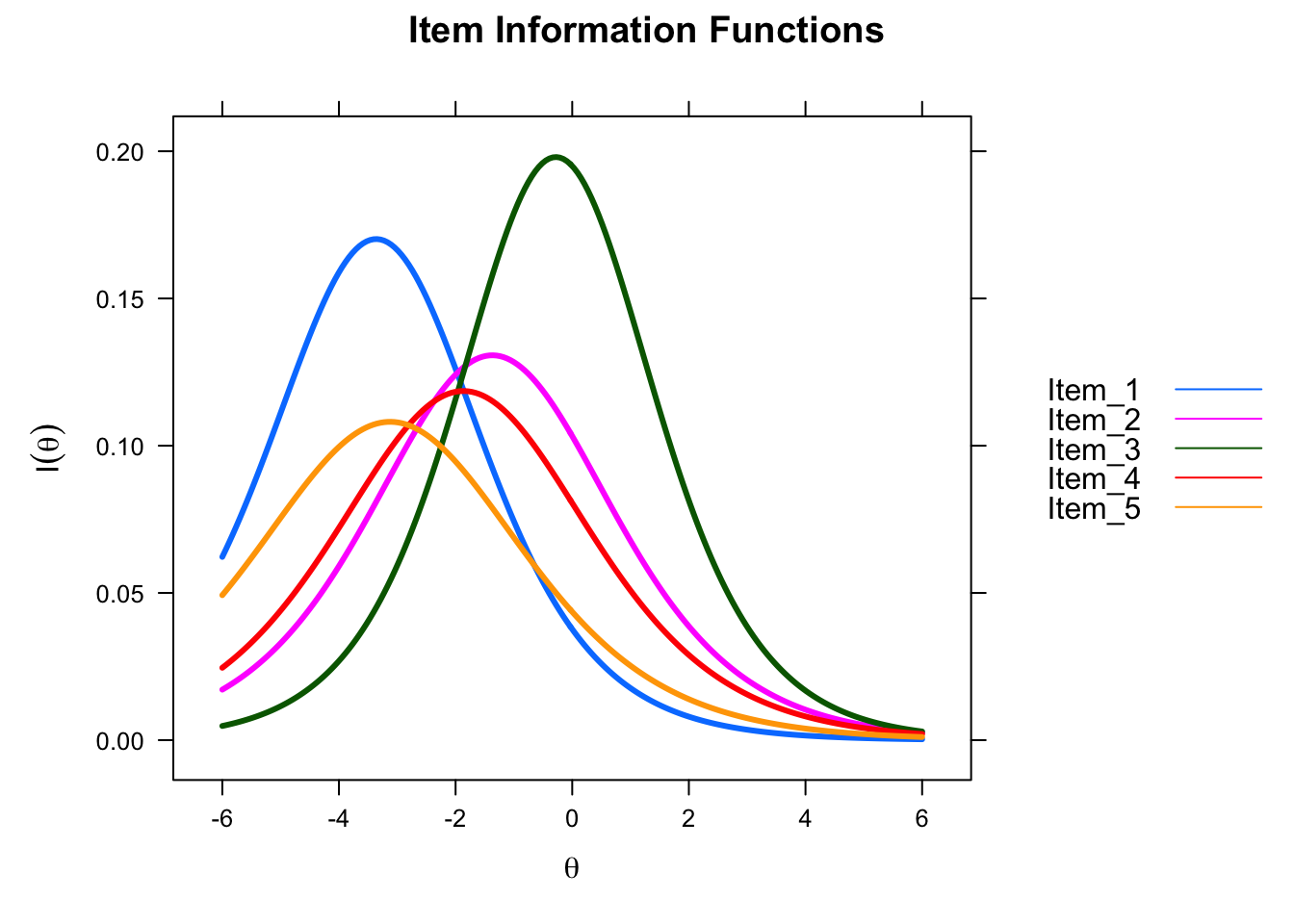
Based on the estimated parameters for every item of a given test, we can compute and plot the amount of information (i.e., the precision to measure an ability level) provided by every item. It is important to note that the amount of information will have its peak on the item's difficulty parameter (\(b_{j}\)), decreasing the amount of information that the item provides with the departure from the \(b_{j}\) estimate.
Relying on the LSAT6 parameter estimates (see Table 4), we can compute the Item Information Function (IIF) for all items using the following equation:
\[\\I_{j}(\theta)\ = \ a^{2}_{j}\ P_{j}(\theta)\ Q_{j}(\theta)\]
The previous equation is suited for 2PLM. For 1PLM, we will fix the discrimination parameter (\(a_{j} = 1\)) in order to simplify the equation.
\[\\I_{j}(\theta)\ = \ P_{j}(\theta)\ Q_{j}(\theta)\]
We can also plot the Item Information Function (IIF) of individual items separately or plot the item information tracelines of several items into a single graphic. In the following plot, we can observe that item 3 is highly informative; its peak is close to \(I_{j}(\theta) = 0.20\). Be aware that item 3 is highly informative around the ability levels above and below zero (\(b_{j} = -0.28\)). However, item 1 will be a better candidate than item 3 if we require an informative item for lower levels of ability (e.g., \(\theta = -3\)).
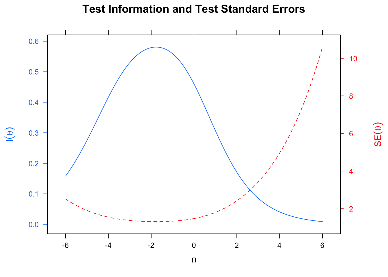
15.5.2 Test Information Function
The Test Information Function (TIF; \(I(\theta)\)) can be defined as the sum of the item information functions of a test. As it is a function, the information (i.e., precision) of a test varies with every value of \(\theta\).
\[\\I(\theta)\ = \ \displaystyle\sum_{j=1}^{J}\ I_{j}(\theta)\]
The value that the TIF yields depends on: (1) the number of items, (2) the parameters \(a_{j}\) (i.e., discrimination) and \(c_{j}\) (i.e., guessing), and (3) the proximity between \(\theta\) and \(b_{j}\). It is important to consider that the concept of Test Information cannot be fully understood without its reciprocal: the Standard Error of the estimate of the ability/trait (\(SE(\theta)\)).
\[\\SE(\theta)\ = \ \frac{1}{\sqrt{I(\theta)}}\]
A test would be best for estimating the ability/trait of the respondents whose \(\theta\) scores fall near the peak of the Test Information Function. Precision of the estimates will decrease when departing from that peak. However, the precision of the test won't be appropriate for \(\theta\) values located below and above the thresholds in which the tracelines of \(I(\theta)\) and \(SE(\theta)\) converge.