14.7 Other reliability coefficients
In this section, we will inspect other reliability coefficients generated with other functions that you can find in the package psych (Revelle, 2018; Revelle & Zinbarg, 2009). Although most reliability coefficients will yield similar values despite the different functions being used, differences might arise due to the different procedures used to estimate these coefficients. In addition to reading the literature on the topic, read the description and details provided in every function that we use in R.
First, we will use the function omega() to estimate both Omega hierarchical (\(\omega_{h}\))---the estimation of the general factor saturation of a test---and Omega total (\(\omega_{t}\))---the estimation of the total reliability of the test. We must set the optional argument nfactors to 2 because those were the number of factors that we extracted in Chapter 13 (Exploratory Factor Analysis).
psych::omega(burnout, nfactors = 2, flip = TRUE)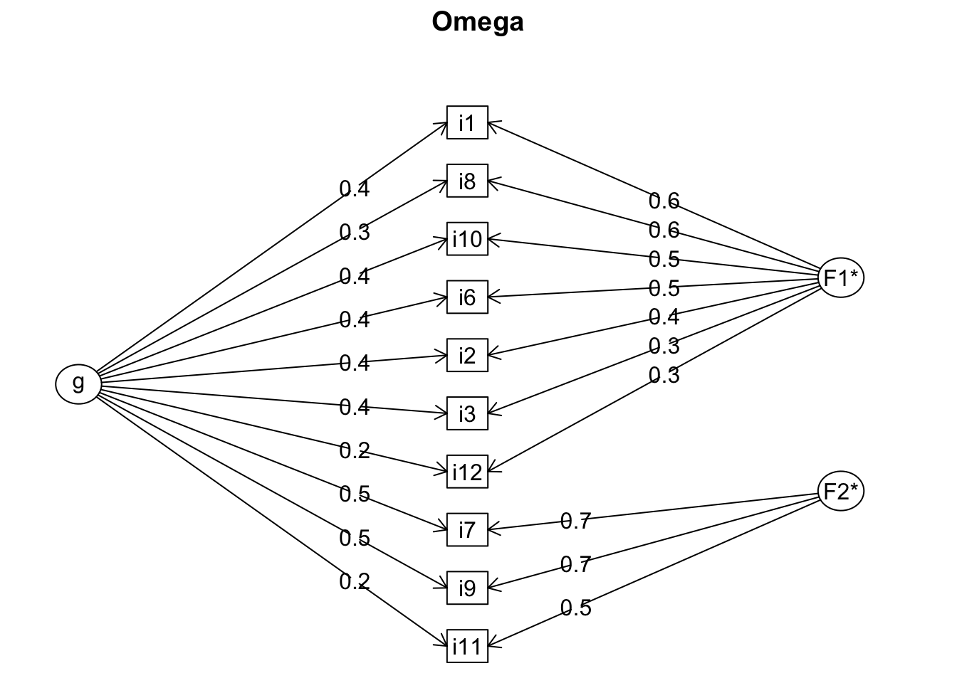
## Omega
## Call: omegah(m = m, nfactors = nfactors, fm = fm, key = key, flip = flip,
##     digits = digits, title = title, sl = sl, labels = labels,
##     plot = plot, n.obs = n.obs, rotate = rotate, Phi = Phi, option = option,
##     covar = covar)
## Alpha:                 0.79
## G.6:                   0.81
## Omega Hierarchical:    0.41
## Omega H asymptotic:    0.49
## Omega Total            0.83
##
## Schmid Leiman Factor loadings greater than  0.2
##        g   F1*   F2*   h2   u2   p2
## i1  0.43  0.62       0.57 0.43 0.33
## i2  0.40  0.45       0.37 0.63 0.43
## i3  0.36  0.31       0.26 0.74 0.49
## i6  0.42  0.50       0.44 0.56 0.41
## i7  0.47        0.66 0.66 0.34 0.34
## i8  0.30  0.56       0.43 0.57 0.21
## i9  0.50        0.65 0.68 0.32 0.37
## i10 0.41  0.53       0.45 0.55 0.37
## i11 0.24        0.45 0.28 0.72 0.20
## i12 0.21  0.27       0.12 0.88 0.37
##
## With eigenvalues of:
##   g F1* F2*
## 1.5 1.6 1.1
##
## general/max  0.92   max/min =   1.4
## mean percent general =  0.35    with sd =  0.09 and cv of  0.26
## Explained Common Variance of the general factor =  0.35
##
## The degrees of freedom are 26  and the fit is  0.16
## The number of observations was  510  with Chi Square =  82.82  with prob <  0.000000077
## The root mean square of the residuals is  0.04
## The df corrected root mean square of the residuals is  0.05
## RMSEA index =  0.065  and the 10 % confidence intervals are  0.05 0.082
## BIC =  -79.28
##
## Compare this with the adequacy of just a general factor and no group factors
## The degrees of freedom for just the general factor are 35  and the fit is  1.32
## The number of observations was  510  with Chi Square =  667.5  with prob <  0.0000000000000000000000000000000000000000000000000000000000000000000000000000000000000000000000000000000000000000000006
## The root mean square of the residuals is  0.19
## The df corrected root mean square of the residuals is  0.21
##
## RMSEA index =  0.188  and the 10 % confidence intervals are  0.176 0.201
## BIC =  449.29
##
## Measures of factor score adequacy
##                                                   g  F1*  F2*
## Correlation of scores with factors             0.66 0.76 0.77
## Multiple R square of scores with factors       0.43 0.58 0.59
## Minimum correlation of factor score estimates -0.13 0.16 0.17
##
##  Total, General and Subset omega for each subset
##                                                  g  F1*  F2*
## Omega total for total scores and subscales    0.83 0.79 0.77
## Omega general for total scores and subscales  0.41 0.30 0.25
## Omega group for total scores and subscales    0.40 0.49 0.52
Omega hierarchical (\(\omega_{h}\)) estimates the general factor saturation of a test. In the burnout data set, the factor loadings were moderate for some items (e.g., items i1 and i8) and low for others (e.g., items i11 and i12). For this reason, Omega hierarchical yields a low value (\(\omega_{h} = .41\)). Be aware that the reliability coefficient estimated with Guttman's \(\lambda_{6}\) (\(G6 = .81\)) tends to be similar to Omega total (\(\omega_{t} = .83\)).
Cronbach's alpha coefficient estimated with the function omega() is .79, whereas the coefficient estimated with the function alpha() yielded a lower value (\(\alpha = .78\)). In case of disagreement, use Cronbach's alpha reliability coefficient estimated with the functions omega() or iclust() (in this example, \(\alpha = .79\)).
We can also inspect the tables (e.g., Schmid Leiman Factor loadings greater than 0.2) to reach the same conclusion in relation to keeping or dropping items. The decision to drop items has to consider the fact that latent variables with less than 3 observable measures (i.e., items) will lead to an unspecified model (Fabrigar et al., 1999).
In the previous example, we produced a plot with the second order factor (g) displayed on the left. On the other hand, the first order factors (Affective and Reward; i.e., factors 1 and 2) were plotted on the right-hand side without an arrow connecting them (both factors were assumed to be uncorrelated or orthogonal). This model is called bifactor, but it is not easily found in psychology. As we discussed in previous sessions, most psychological constructs tend to be correlated to each other. Indeed, in the session Exploratory Factor Analysis we found that the two factors extracted from the Job Burnout Scale were correlated (interfactor correlation, \(r = .37\)). Consequently, we cannot use here a bifactor approach (i.e., factors are independent) to visualize the internal structure of the Job Burnout Scale, but a hierarchical approach. In the next visualization, we will be able to observe that the path diagram shows two first order latent variables (factors 1 and 2) and one second order factor (g).
The argument sl refers to how we would like to plot the results (i.e., using the Schmid Leiman solution or not). The defaulted model assumes that the factors are independent (not correlated). The default option sets this argument to TRUE. Thus, by setting the argument sl to FALSE, we will plot a hierarchical solution, assuming that the first order latent variables are correlated and that they also reflect the higher order latent variable (g).
my.omega <- psych::omega(burnout, nfactors = 2, sl = FALSE,
                         rotate = 'oblimin', fm = 'ml', digits = 2,
                         option = 'equal', flip = TRUE)
In the previous R code, we stored the computations executed with the function omega() in the object my.omega. We specified the number of factors (nfactors = 2) and the estimation of a hierarchical model (correlated factors; sl = FALSE). Likewise, we used the rotation method oblimin for correlated factors and the estimation method ml (maximum likelihood). For two factors, we had to specify equal loadings for both factors. Finally, we flipped the items negatively correlated to the general factor.
The function omega.diagram() enables us to use the object my.omega to get the hierarchical plot with some interesting modifications. For example, we can set the labels of the factors (flabels = c('Affective', 'Reward')). We can also specify the cutoff point for the loadings (cut = .30), increase or decrease the font size (cex) or the size of the round boxes of the factors (e.size).
omega.diagram(my.omega, sl = FALSE, flabels = c('Affective', 'Reward'),
              cut = .3, digits = 2, e.size = .15, cex = 1.2, adj = 2,
              main = ' \n Hierarchical Omega (Burnout dataset)')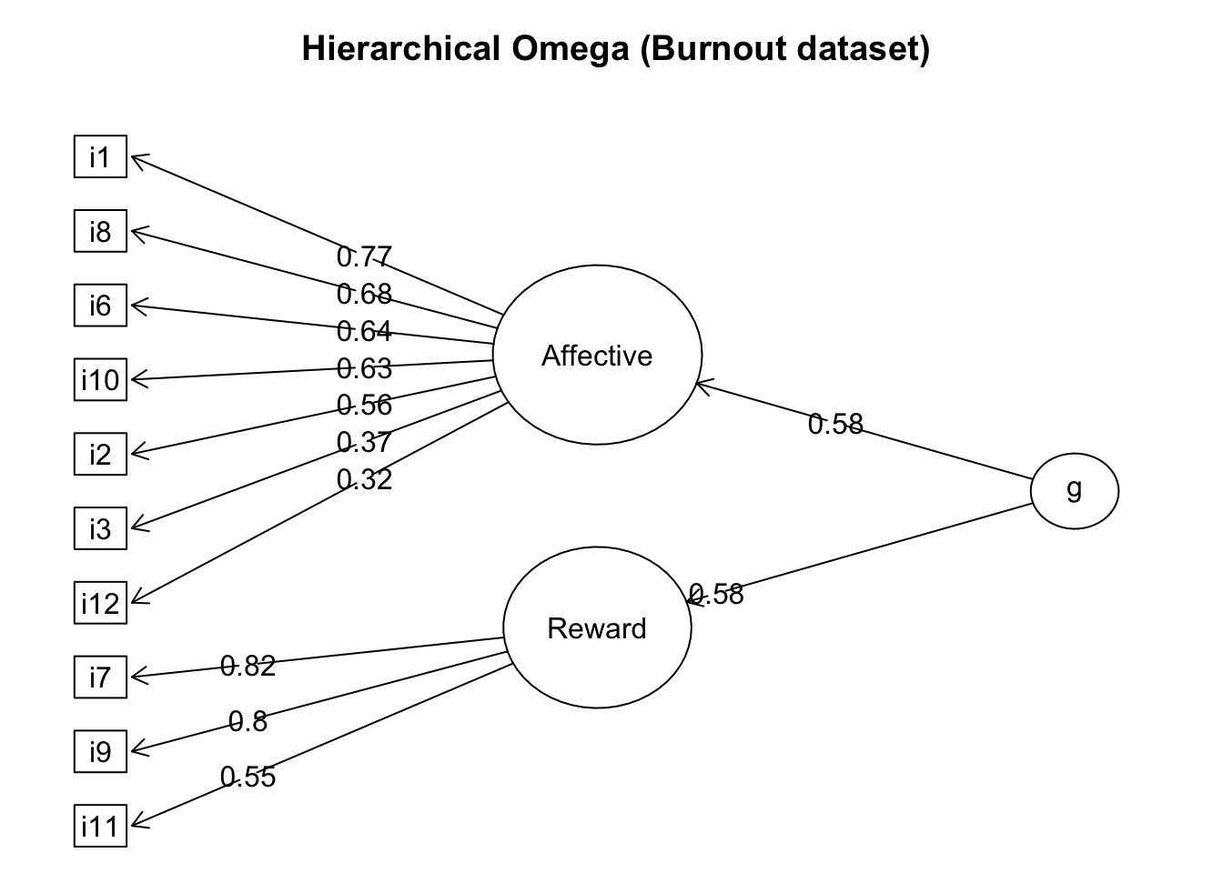
The function guttman() estimates Guttman's Lambdas (\(\lambda_{1}\) to \(\lambda_{6}\)). Please, remember that \(\lambda_{3}\) provides the same reliability estimation as Cronbach's alpha coefficient (\(\alpha\)). Beta (\(\beta\)) is a reliability coefficient that looks for the worst split half to generate the coefficient of reliability (Revelle & Zinbarg, 2009). Consequently, beta (\(\beta\)) is an estimator that yields a low reliability value (i.e., a lower bound of reliability). However, the best estimation of beta (\(\beta\)) is computed with the function iclust() that will be explained below.
psych::guttman(burnout)
## Call: psych::guttman(r = burnout)
##
## Alternative estimates of reliability
##
## Guttman bounds
## L1 =  0.71
## L2 =  0.8
## L3 (alpha) =  0.79
## L4 (max) =  0.85
## L5 =  0.77
## L6 (smc) =  0.81
## TenBerge bounds
## mu0 =  0.79 mu1 =  0.8 mu2 =  0.8 mu3 =  0.8
##
## alpha of first PC =  0.8
## estimated greatest lower bound based upon communalities=  0.87
##
## beta found by splitHalf  =  0.6
The function splitHalf() computes the split half of the test and provides an estimation of \(\lambda_{3}\), \(\lambda_{4}\), and \(\lambda_{6}\). The estimation of \(\beta\) as the minimum split half reliability is important because it contrasts sharply with \(\lambda_{4}\) (i.e., the greatest split half reliability).
psych::splitHalf(burnout)
## Split half reliabilities
## Call: psych::splitHalf(r = burnout)
##
## Maximum split half reliability (lambda 4) =  0.85
## Guttman lambda 6                          =  0.81
## Average split half reliability            =  0.79
## Guttman lambda 3 (alpha)                  =  0.79
## Guttman lambda 2                          =  0.8
## Minimum split half reliability  (beta)    =  0.6
## Average interitem r =  0.27  with median =  0.27
The function iclust() finds the overall correlation matrix to combine the two most similar items into a new (composite) item. Then, it computes the correlation of this new item with the remaining items and repeats this process until the worst split half correlation (\(\beta\)) stops increasing.
Here, beta (\(\beta\)) will tend to coincide with omega hierarchical (\(\omega_{h}\)) as both reliability coefficients estimate the general factor saturation (Revelle, 2018). In case of disagreements among the values generated for beta (\(\beta\)) in other functions included in the package psych, always report iclust()'s original beta (\(\beta = .48\)).
psych::iclust(burnout, plot = TRUE, reverse = TRUE)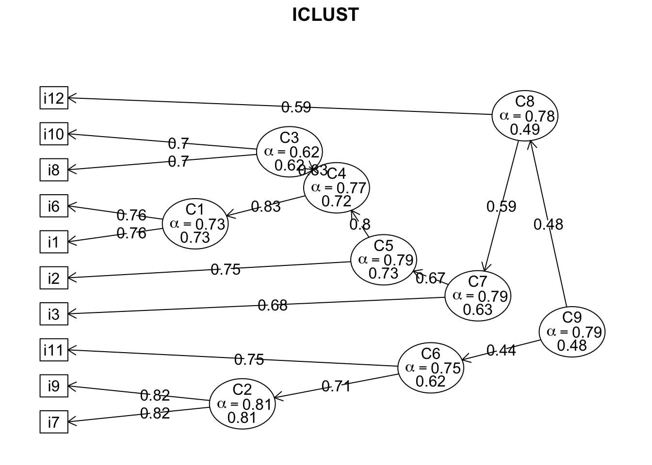
## ICLUST (Item Cluster Analysis)
## Call: psych::iclust(r.mat = burnout, reverse = TRUE, plot = TRUE)
##
## Purified Alpha:
## [1] 0.79
##
## G6* reliability:
## [1] 1
##
## Original Beta:
## [1] 0.48
##
## Cluster size:
## [1] 10
##
## Item by Cluster Structure matrix:
##     [,1]
## i1  0.65
## i2  0.60
## i3  0.51
## i6  0.63
## i7  0.57
## i8  0.47
## i9  0.62
## i10 0.62
## i11 0.26
## i12 0.32
##
## With eigenvalues of:
## [1] 2.9
##
## Purified scale intercorrelations
##  reliabilities on diagonal
##  correlations corrected for attenuation above diagonal:
##      [,1]
## [1,] 0.79
##
## Cluster fit =  0.65   Pattern fit =  0.93  RMSR =  0.12